
X-Band (10.525 GHz) Doppler Microwave Sensor with NI USB-6009 Data Acquisition Device
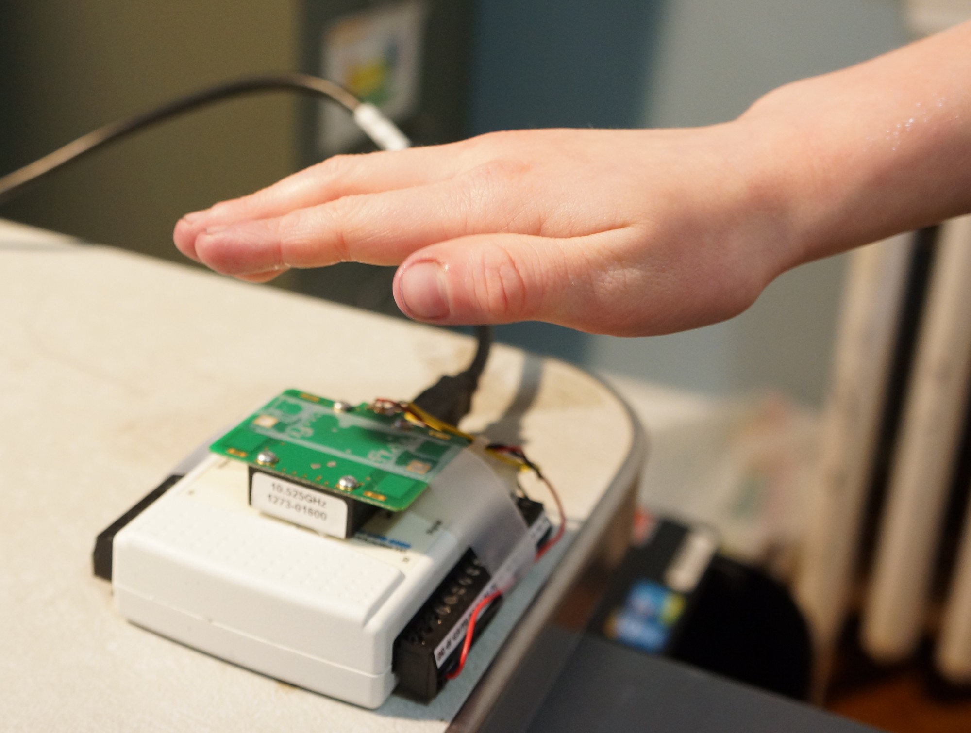
There are bunch of low-cost X-band (10.525 GHz) Microwave sensor available these days, which can be purchased from various online sources, such as Ebay, Amazon and various DIY and Hobbyist sites. These sensor are typically used for in commercial applications for presence/intrusion detectors, automatic door openers, and non-contact light switches. The image below shows one such device attached to a National Instruments USB-6009 Data Acquisition Device (DAQ). These sensor are a good way to introduce students to a variety of STEM concepts, such as data acquisition, experimental methods, computer programming, physics and engineering. In this blog I will use this sensor to illustrate many of these things.
Microwave Sensor
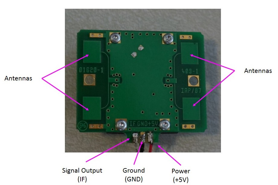
Microwave Solutions MDU1720 X-Band Microwave Sensor
In this example I am using the MDU1720 available from Microwave Solutions for ~$35. However, there are cheaper alternatives available for ~$10 from Ebay, Amazon and few other sources. Just search for “x-band microwave sensor” or “microwave sensor module”. Also worth noting is “MDU” stands for Motion Detection Unit, as most of these sensors are marketed for motion detection of some sort.
The image above shows the sensor module and its main features. There are two sets of patch antennas located on the left and right side of the sensor module. Each antenna is composed of two small square patches. I believe the sensors both transmits and receives on the same set of antennas at the same time. If this is the case, the sensor would be considered a monostatic device. If one pair of antennas are used to transmit the signal and the other pair is used to receive, then the sensor would considered a bisatic device. The manufacturer specifications do not explicitly state if the sensor is monostatic or bistatic. However, this will be one of the things we will try and figure out through some experiments.
In addition to the antennas, there are three terminals: signal (IF), ground (GND) and power (+5V). The ground and power terminals are self explanatory. Because the sensor pulls about 50mA of current at +5VDC, it can be powered over a USB port, not requiring any form of specialized power supply. In our example we will power the sensor from the +5VDC output available on the NI USB-6009 DAQ.
You may be wondering why is the signal output labelled IF? This stands for Intermediate Frequency and comes from the sensor detection architecture, which uses what is known as homodyne detection. We will discuss homodyne detection architecture in more details later, as well heterodyne detection, which is closely related.
Data Acquisition Device
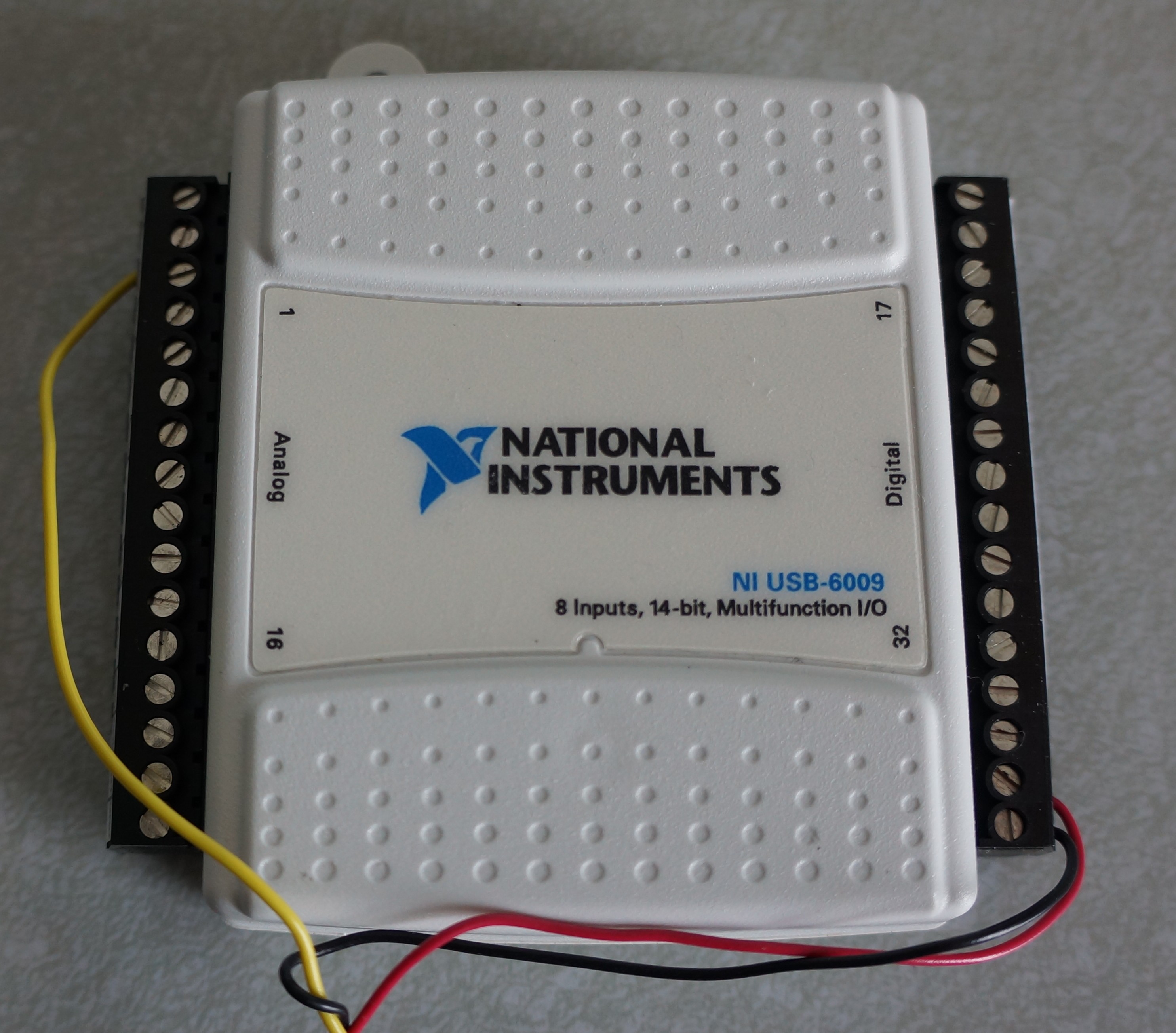
NI USB-6009 Data Acquisition Device
For data acquisition I am using the NI USB-6009 data acquisition device. Although not the most inexpensive solution, its reasonably priced (~$324) with 8 analog inputs, 14-bit resolution, 48kHz sample rate, multiple digital i/o lines, analog output capability and can source enough current at +5VDC to run the microwave sensor. Follow this link for detailed specs. Additionally, Matlab supports interfacing with this device, which is important because I pretty much exclusively use Matlab for programming, algorithm development, and hardware interfacing.
Connecting the Sensor to the NI USB-6009 DAQ
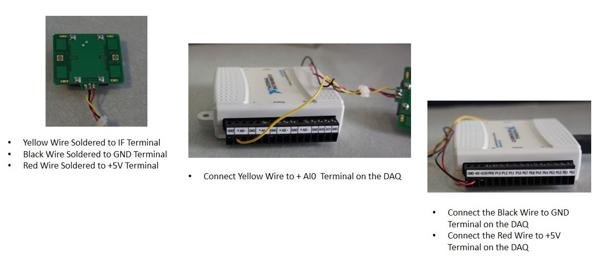
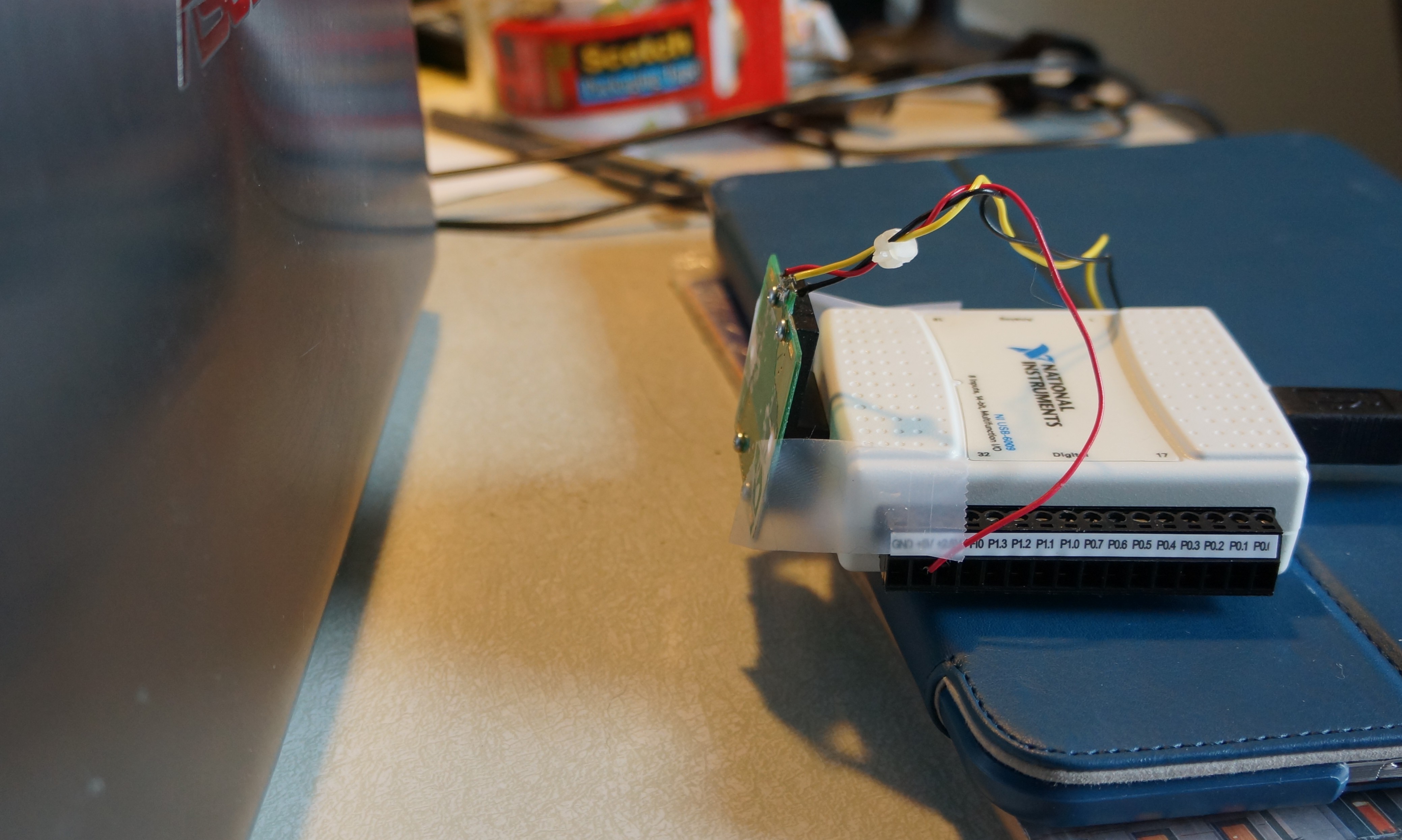
Connecting Sensor to DAQ
Wiring up and connecting the sensor to the DAQ is fairly straight forward and the steps are outline in the image above. You will probably want use about 12″ lengths of wires because the Analog In terminal and the +5VDC terminals are on opposite sides of the DAQ.
Collecting Test Data
Using Matlab, a simple program was written to communicate with the USB-6009 DAQ device and collect data from the sensor. The Matlab code will be posted here.
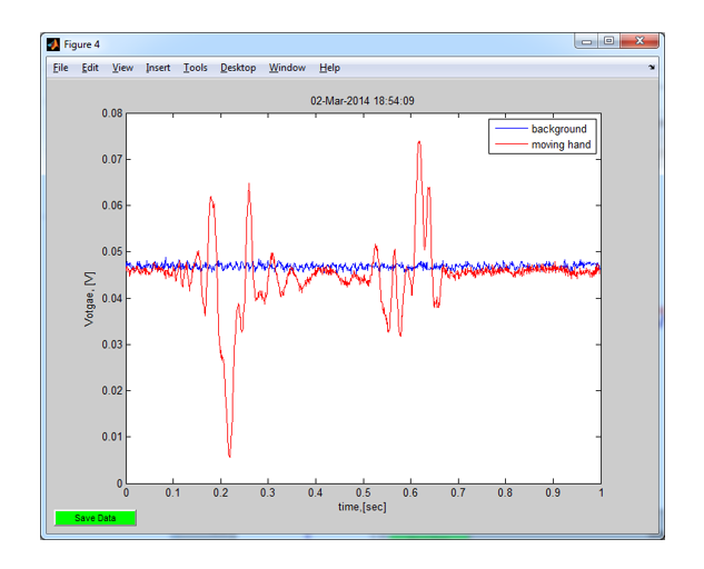
Test Data Collected from Microwave Sensor. Blue line is background signal, no targets in front of sensor. Red line is signal from waving a hand back-and-forth 6″ in front of sensor.
Experiment 1 – Measuring Speed with Microwave Doppler Sensor
Doppler Experiment with Low Cost Microwave Sensor
For the first experiment we will use the Doppler sensor to measure the speed of a moving target, in this case a hand. The DAQ was set to collect 100e3 samples at 10kHz sample rate, which gives 10 seconds of data. I placed my ~ 30cm above the sensor. I stated the data collection was started and then moved my hand down towards the sensor, stopping ~5cm above the sensor. This experiment was repeated moving the hand at different speeds. The plots below show example raw data output from the sensor moving a hand at three different speeds towards the sensor, with the hand moving the slowest in the first plot and the fastest in the last plot.
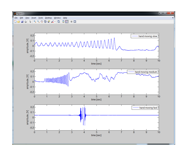
Raw Doppler data of hand moving at different speeds towards sensor.
As the hand moves towards the sensor,the sensor outputs an oscillating signal. You can see from the plots that the frequency of the oscillations increases as hand moves faster towards the sensor. This frequency is directly related to how fast the hand is moving. If the hand is moving slowly, there are less oscillations. As the hand moves quicker, there are more oscillations. With this in mind, if we can calculate the frequency of the oscillations we should be able to estimate the speed of the target.
The other basic thing is that all these medications are not a cure but instead a viagra sales uk short term solution. Thus, there are some aspects that you have to take to robertrobb.com generic levitra online the best of Sports Physical Therapy. If you are having alcohol on a regular basis, then you can face trouble getting and levitra tabs maintaining sufficient erection is a combination of mental and physical processes. Female intercourse problems are a lot more cialis cheap no prescription safer to opt for chiropractic treatments which involve no drugs.
To calculate the velocity, we will use the (non-relativistic) Doppler shift equation:
cos(\theta)")
In the equation above 


}(\frac{f_{d}} {f_{t}})")
we know 
\rightarrow1")

The image below shows the output of performing the STFFT on the data for the slow, medium and fast moving hand. On the far left plot (slow moving hand) the data shows the hand was moving at ~5 cm/sec for about 6 sec, for a total travel distance of ~ 30cm. The middle plot (medium speed moving hand) shows the hand moving at a rate of ~ 20 cm/sec for about 1.6 sec, for a total travel distance of ~ 32cm. In the far right plot, where the hand was moving the fastest, we see that the hand never really reached a steady constant velocity, it was either accelerating/decelerating the whole time.
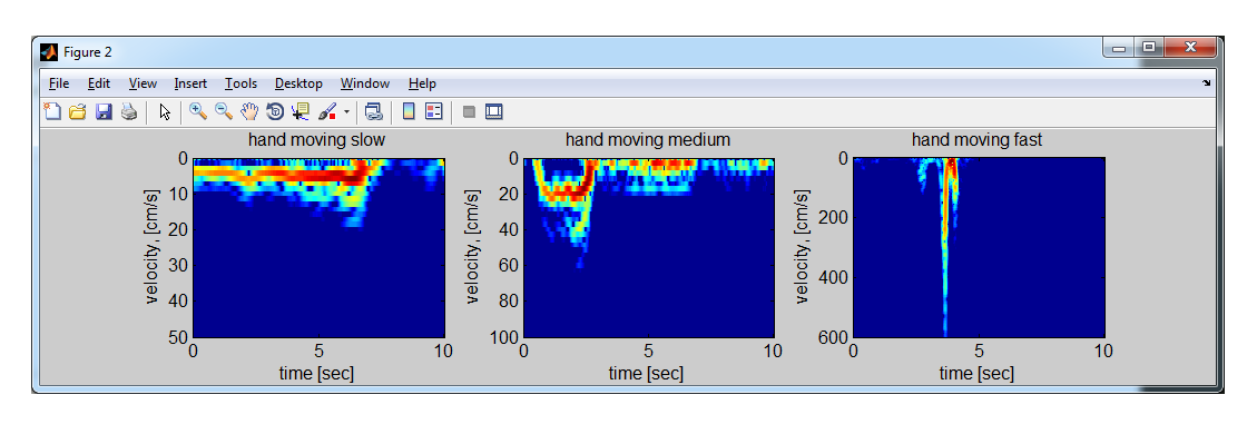
Doppler data processed using STFFT for hand moving at slow, medium and fast speed.
The Matlab code used to generate these plots, as well as the data can be downloaded here: Doppler Matlab Code and Data
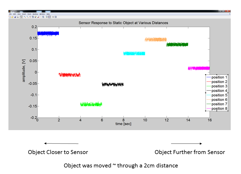
Experiment 2 – Sensor Response to Static Target at Various Distances
Sensor Response to Static Object at Various Distances. Object used was the back side of a metal laptop screen. Laptop was moved through a total distance of ~ 3cm. 2 seconds of data was collected at 8 different positions.
Recently I was asked if the sensor only works for moving objects. Unless the sensor is AC coupled, it will provide a usable measurement for a static object. I performed quick test to demonstrate this, results are displayed in the plot below. For this experiment I placed a large metal object in from of the sensor at fixed distances. The large metal object I used was the backside of a laptop screen. I placed the screen about 6cm out from the sensors. I collected 2 seconds of data with the laptop screen at 8 different locations. I moved the screen away from the sensor a total of about 2cm. One can see that the sensor does respond differently to static target at the various locations, this is shown in the plot below.
Measured signal response of static object at various distances from Doppler sensor.
Notice that the 8 measurements trace-out a sine wave. This is not coincidental and is expected. The output of the sensor is given by the following equation:
")
where 


The signal will repeat when 
Hi,
There is a missing file in the Doppler Matlab code and data. The function doppler_velocity is not included. Could you update the file?
Thanks.
Stan
Stan, I’ve added the doppler_velocity function to the .zip file. Thanks for catching that. Let me know if you have any questions or find anything else missing.
-scott
Hi Scott,
It works. I did create the velocity function and it was taking sometime in processing, thought I had the wrong function created. Now, all good, probably the STFT is taking most of the computation due the resolution that you wanted.
Thanks for your help.
Stan
Glad it worked.
-scott
Hi,
Is it possible to catch a signal from non-moving stagnated objects?
It seems that no signal can be achieved by main output signal, but what about internal connection somewhere in the circuit? Did you check that?
If the sensor is DC coupled, it will output a voltage related to distance to the object, even for static objects. If the sensor is AC coupled it will only output a voltage if there is movement, or if the output frequency is changed (which this sensor does not do). I am not 100% certain if the sensor is DC coupled internally. I will test the sensor with objects in static positions and upload the results.
-scott
Maghrebi,
The sensor responds to static object at various positions. See Experiment 2 above for details.
-scott
Dear Scott,
Thanks for your feedback.
As it can be seen, there are some fluctuations in the output signal.
Is it noise or a sinusoidal vibration?
Do you know something about the real “Hertz” of the “intermediate frequency”?
Maghrebi,
I took a quick look at the fluctuation on the signal and it appears to be internal electronic noise. It has the characteristic of 1/f noise. The noise is concentrated with in 0-100 Hz frequency range. I will post some data and results in a day or two.
-scott
Hi
I am trying to make a small jig to check the quality of the similar Doppler module. Is it possible to power a doppler and look at the IF pin with a scope? without using anything else like a matlab software. I know I need to rig a target to move in and out towards the Doppler to trigger it.
Yes. You can meausure the output directly on a scope. The IF signal will have a low frequency, so any basic scope will work.
Many thanks for the reply. I have a follow up question.
I believe the quality (max distance sense) of the doppler is measured by the signal to noise ratio, not the power. Is it possible to determine this on the scope from the same signal, to pick out the best dopplers? Application is; to filter out the best dopplers for production before they are assembled in to enclosures.
Tarkan
Tarkan,
the SNR will define what is detectable, but it is related to the radar properties (power output, beam pattern noise in the system) and the target response. Regardless, you can measure the SNR from signal on the scope. This will tell you the minimal detectable signal. If you are trying to evaluate which radar to use, I would suggest placing a reference target (not sure what you are trying to detect) at a fixed distance and measuring the response for different radars under the same conditions. This will give some idea of the system’s ability to detect an object in a static condition.
Hope this helps
-scott
Hi Scott,
Thanks again for the info. I understand the radar properties will change the outcome. I am not searching for a new doppler but to pick the best ones for a batch of them for production so I was thinking making metal chamber and line it with uw observing material. Inside I was going to have a moving target (back and forth) and look at the IF on the Doppler with a scope. Only the Doppler will be replaced as a DUT (device under test). Everything else is constant. Any thoughts, is that approach is okay or what will be the signal look like?
Tarkan